Signal Processing with NumPy II - Image Fourier Transform : FFT & DFT
The DFT (Discrete Fourier Transform) is defined as $$A_k = \sum_{m=0}^{n-1} a_m exp\{ -2\pi i \frac{mk}{n} \} \quad\quad k=0,...,n-1.$$ The DFT is in general defined for complex inputs and outputs, and a single-frequency component at linear frequency f is represented by a complex exponential $a_m = exp\{2\pi i f m \Delta t \}$, where $\Delta t$ is the interval for sampling.
Here are the NumPy's fft functions and the values in the result:
- $A=fft(a,n)$
$A[0]$ contains the zero-frequency term which is the mean of the signal. It is always purely real for real inputs.
$A[1:n/2]$ contains the positive-frequency terms.
$A[n/2+1:]$ contains the negative-frequency terms in the order of decreasing negative frequency $A[n/2]$ represents both positive and negative Nyquist frequency for an even number of input points. It is also purely real for real input.
$A[(n-1)/2]$ contains the largest positive frequency for an odd number of input points.
$A[(n+1)/2]$ contains the largest negative frequency.
- $fftfreq(n)$
returns an array giving the frequencies of corresponding elements in the output. - $fftshift(A)$
shifts transforms and their frequencies to put the zero-frequency components in the middle. - $ifftshift(A)$
undoes the shift done by $fftshift(A)$.
When $a$ is a time-domain signal in $A = fft(a)$
- $abs(A)$ : its amplitude spectrum
- $\{ abs(A) \}^2$ : its power spectrum
- $angle(A)$ : its phase spectrum
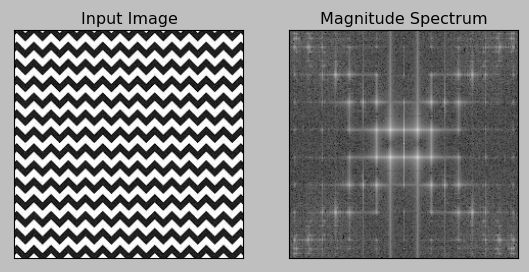
import cv2
import numpy as np
from matplotlib import pyplot as plt
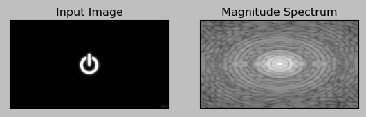
img = cv2.imread('xfiles.jpg',0)
f = np.fft.fft2(img)
fshift = np.fft.fftshift(f)
magnitude_spectrum = 20*np.log(np.abs(fshift))
plt.subplot(121),plt.imshow(img, cmap = 'gray')
plt.title('Input Image'), plt.xticks([]), plt.yticks([])
plt.subplot(122),plt.imshow(magnitude_spectrum, cmap = 'gray')
plt.title('Magnitude Spectrum'), plt.xticks([]), plt.yticks([])
plt.show()
The '2' in $fft2()$ indicates that we're using 2-D fft. The $fft2()$ provides us the frequency transform which will be a complex array. Its first argument is the input image, which is grayscale. Second argument is optional which decides the size of output array.
If we use interactive shell, the $f$ looks like this:
>>> f.shape
(194, 259)
We can see $fft2()$ returns a complex array:
>>> f
array([[ 842784.00000000    +0.j        , -517752.56442341 -3696.20384447j,
          91285.56071617 +4921.45028062j, ...,
         -46601.18635079 -4814.84303878j,   91285.56071617 -4921.45028062j,
        -517752.56442341 +3696.20384447j],
       [ 123232.14686474+22090.02037498j,    -856.26680325 +9182.45344817j,
        -136191.25175358-51466.45725155j, ...,
          71425.20605824+14903.15993681j, -158452.77640809-31181.5124568j ,
          -3060.27297752+19352.80159523j],
       [ -36743.19890402-14189.86326576j,   28037.83427034+45830.48236385j,
          -5472.34460100  +751.10794956j, ...,
         -17431.81487318-56998.95644394j,  -27977.32223743-17396.44346126j,
          55230.60393901+23180.07097916j],
       ...,
       [-107889.78457811+41341.29205987j,   15392.03432529 +8349.74473343j,
          61145.55093605-59049.02715308j, ...,
          40527.83113022+19449.36030634j,   73913.64630259-52167.06835863j,
          -7173.60813531 +8395.54640485j],
       [ -36743.19890402+14189.86326576j,   55230.60393901-23180.07097916j,
         -27977.32223743+17396.44346126j, ...,
         -29773.75673263+47038.82271301j,   -5472.34460100  -751.10794956j,
          28037.83427034-45830.48236385j],
       [ 123232.14686474-22090.02037498j,   -3060.27297752-19352.80159523j,
        -158452.77640809+31181.5124568j , ...,
          58992.94700240 +3233.35145839j, -136191.25175358+51466.45725155j,
           -856.26680325 -9182.45344817j]])
We did $ffshift()$ because we want to place the zero-frequency component to the center of the spectrum. In other words, once we got the result, zero frequency component (DC component) will be at top left corner. Because we want to bring it to center, we needed to shift the result by $\frac{n}{2}$ in both the directions using $np.fft.fftshift()$.
Once we found the frequency transform, we can find the magnitude spectrum:
magnitude_spectrum = 20*np.log(np.abs(fshift))
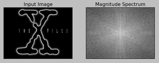
Now we can see more whiter region at the center showing we have more low frequency content.
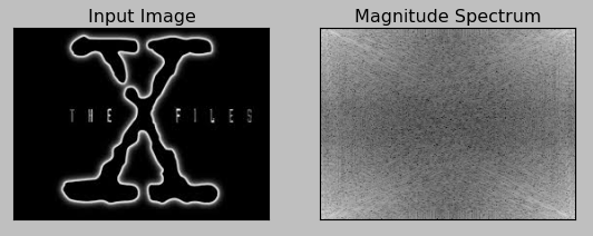
If we undo the shift using $ffshift()$:
f = np.fft.fft2(img)
fshift = np.fft.fftshift(f)
fshift = np.fft.ifftshift(fshift)
The picture will look like this:
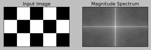
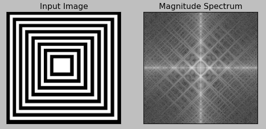
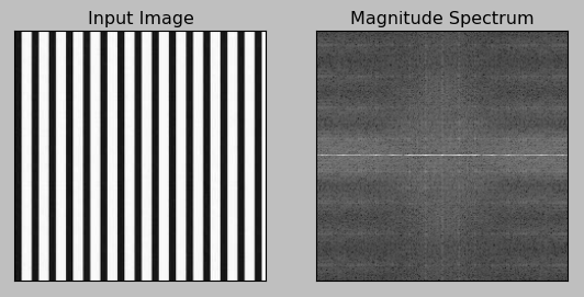
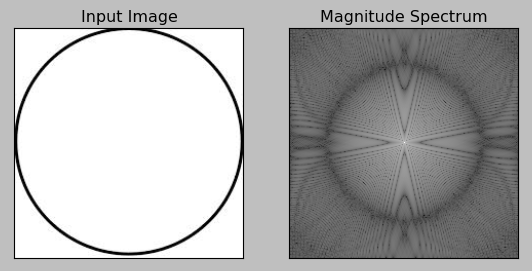
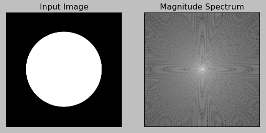
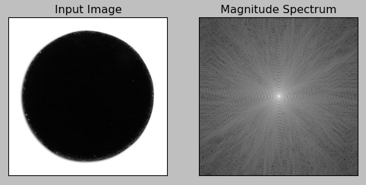
Here are more fft samples:
We found the frequency transform for an image in the previous section. So, now we can do some operations in frequency domain, like high pass filtering (HPF) and reconstruct the image using inverse DFT.
We can simply remove the low frequencies by masking with a rectangular window of size 60x60. Then, apply the inverse shift using $ifftshift()$ so that DC component again come at the top-left corner. Then, find inverse FFT using $ifft2()$ function. The result, again, will be a complex number. We can take its absolute value.
The DFT (Discrete Fourier Transform) is defined as: $$A_k = \sum_{m=0}^{n-1} a_m exp\{ -2\pi i \frac{mk}{n} \} \quad\quad k=0,...,n-1.$$ The inverse DFT is defined as this: $$A_m = \frac{1}{n} \sum_{k=0}^{n-1} A_k exp\{ 2\pi i \frac{mk}{n} \} \quad\quad m=0,...,n-1.$$
import cv2
import numpy as np
from matplotlib import pyplot as plt

img = cv2.imread('xfiles.jpg',0)

# fft to convert the image to freq domain
f = np.fft.fft2(img)

# shift the center
fshift = np.fft.fftshift(f)

rows, cols = img.shape
crow,ccol = rows/2 , cols/2

# remove the low frequencies by masking with a rectangular window of size 60x60
# High Pass Filter (HPF)
fshift[crow-30:crow+30, ccol-30:ccol+30] = 0

# shift back (we shifted the center before)
f_ishift = np.fft.ifftshift(fshift)

# inverse fft to get the image back
img_back = np.fft.ifft2(f_ishift)

img_back = np.abs(img_back)

plt.subplot(131),plt.imshow(img, cmap = 'gray')
plt.title('Input Image'), plt.xticks([]), plt.yticks([])
plt.subplot(132),plt.imshow(img_back, cmap = 'gray')
plt.title('Image after HPF'), plt.xticks([]), plt.yticks([])
plt.subplot(133),plt.imshow(img_back)
plt.title('Fianl Result'), plt.xticks([]), plt.yticks([])

plt.show()
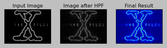
The result shows High Pass Filtering (HPF) is an edge detection operation. This also shows that most of the image data is present in the Low frequency region of the spectrum.
If we watch the result more closely, especially the last image, we can see some artifacts which shows some ripple like structures there, and it is called ringing effects. It is caused by the rectangular window we used for masking. This mask is converted to sine shape which causes this problem. So rectangular windows is not used for filtering. Better option is Gaussian Windows.
Now that we know how to find DFT, IDFT etc. in Numpy. So, let's do it with OpenCV but in next chapter.
OpenCV 3 Tutorial
image & video processing
Installing on Ubuntu 13
Mat(rix) object (Image Container)
Creating Mat objects
The core : Image - load, convert, and save
Smoothing Filters A - Average, Gaussian
Smoothing Filters B - Median, Bilateral
OpenCV 3 image and video processing with Python
OpenCV 3 with Python
Image - OpenCV BGR : Matplotlib RGB
Basic image operations - pixel access
iPython - Signal Processing with NumPy
Signal Processing with NumPy I - FFT and DFT for sine, square waves, unitpulse, and random signal
Signal Processing with NumPy II - Image Fourier Transform : FFT & DFT
Inverse Fourier Transform of an Image with low pass filter: cv2.idft()
Image Histogram
Video Capture and Switching colorspaces - RGB / HSV
Adaptive Thresholding - Otsu's clustering-based image thresholding
Edge Detection - Sobel and Laplacian Kernels
Canny Edge Detection
Hough Transform - Circles
Watershed Algorithm : Marker-based Segmentation I
Watershed Algorithm : Marker-based Segmentation II
Image noise reduction : Non-local Means denoising algorithm
Image object detection : Face detection using Haar Cascade Classifiers
Image segmentation - Foreground extraction Grabcut algorithm based on graph cuts
Image Reconstruction - Inpainting (Interpolation) - Fast Marching Methods
Video : Mean shift object tracking
Machine Learning : Clustering - K-Means clustering I
Machine Learning : Clustering - K-Means clustering II
Machine Learning : Classification - k-nearest neighbors (k-NN) algorithm
Ph.D. / Golden Gate Ave, San Francisco / Seoul National Univ / Carnegie Mellon / UC Berkeley / DevOps / Deep Learning / Visualization