Matlab Tutorial : Digital Image Processing 4 - Grayscale Image II (Data type and bit-plane)

There are one thing to keep in mind when we process images: data type. Is my image in uint8 or double?

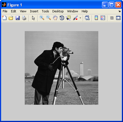
One of the most frequent issues caused by the data type is imshow(). We converted the image to double to do something with the image, and now we want to draw it. Here is an example using the same image : cameraman.tif

img = imread('cameraman.tif');
img_d = double(img);
% ... played with the image, now we want to display it
imshow(img_d);

Let's see what we got:

All white. When I check the pixel values of img_d, the intensities are all in 1-255 range. So, what went wrong?

The imshow() has two function overloading. It takes image with type uint8 as it ranges between [0, 255], and takes image with type double as it ranges between [0, 1]. So, in our case, every pixel with over 1 is considered saturated, and that's why we got white cameraman.

So, we need to scale it to [0,1] range:

img = imread('cameraman.tif');
img_d = double(img);
imshow(img_d/255);

Or better:

img = imread('cameraman.tif');
img_im2d = im2double(img);
imshow(img_im2d);   % img_id2d in [0,1]

Or probably the safest:

img = im2double(imread('cameraman.tif'));
imshow(img);        % img in [0,1]

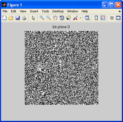
With mod() operation, we can extract a bit-plane image. The mod(img,2) gives us either 0 or 1:

img = imread('cameraman.tif');
img = double(img);
bp0 = mod(img,2);
imshow(bp0);
title('bit-plane 0'); 

For the next bit-plane, basically we do the same operation except we do it after shifting the bit using floor():

bp1 = mod(floor(img/2),2);

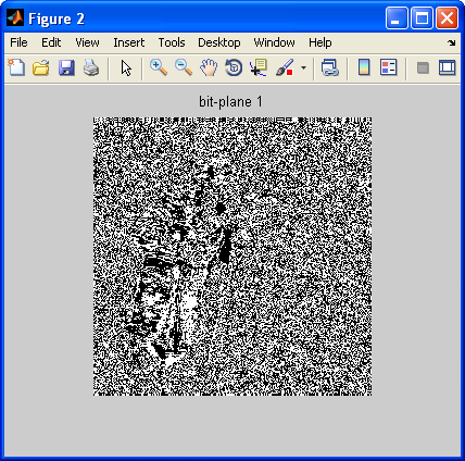
Here is the images for all bit-planes:

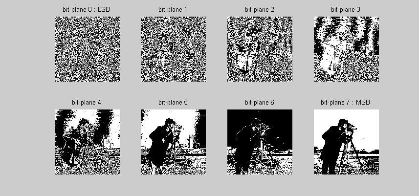
We can see the LSB contributes the least while the MSB contgributes the most!

Here is the script used for the picture above:

img = imread('cameraman.tif');
img = double(img);
bp0 = mod(img,2);
bp1 = mod(floor(img/2),2);
bp2 = mod(floor(img/4),2);
bp3 = mod(floor(img/8),2);
bp4 = mod(floor(img/16),2);
bp5 = mod(floor(img/32),2);
bp6 = mod(floor(img/64),2);
bp7 = mod(floor(img/128),2);

subplot(241);imshow(bp0);title('bit-plane 0 : LSB');
subplot(242);imshow(bp1);title('bit-plane 1');
subplot(243);imshow(bp2);title('bit-plane 2');
subplot(244);imshow(bp3);title('bit-plane 3');
subplot(245);imshow(bp4);title('bit-plane 4');
subplot(246);imshow(bp5);title('bit-plane 5');
subplot(247);imshow(bp6);title('bit-plane 6');
subplot(248);imshow(bp7);title('bit-plane 7 : MSB');

We can put together all the extracted bit-planes and get the original image back:

img = imread('cameraman.tif');
img = double(img);
bp0 = mod(img,2);
bp1 = mod(floor(img/2),2);
bp2 = mod(floor(img/4),2);
bp3 = mod(floor(img/8),2);
bp4 = mod(floor(img/16),2);
bp5 = mod(floor(img/32),2);
bp6 = mod(floor(img/64),2);
bp7 = mod(floor(img/128),2);

bp_all = 2*(2*(2*(2*(2*(2*(2*bp7+bp6)+bp5)+bp4)+bp3)+bp2)+bp1)+bp0;

subplot(241);imshow(bp0);title('bit-plane 0 : LSB');
subplot(242);imshow(bp1);title('bit-plane 1');
subplot(243);imshow(bp2);title('bit-plane 2');
subplot(244);imshow(bp3);title('bit-plane 3');
subplot(245);imshow(bp4);title('bit-plane 4');
subplot(246);imshow(bp5);title('bit-plane 5');
subplot(247);imshow(bp6);title('bit-plane 6');
subplot(248);imshow(bp7);title('bit-plane 7 : MSB');

figure, imshow(uint8(bp_all));