scikit-learn : Decision Tree Learning I - Entropy, Gini, and Information Gain
From wiki
Decision tree learning uses a decision tree as a predictive model which maps observations about an item to conclusions about the item's target value.
It is one of the predictive modelling approaches used in statistics, data mining and machine learning. Tree models where the target variable can take a finite set of values are called classification trees. In these tree structures, leaves represent class labels and branches represent conjunctions of features that lead to those class labels. Decision trees where the target variable can take continuous values (typically real numbers) are called regression trees.
In decision analysis, a decision tree can be used to visually and explicitly represent decisions and decision making. In data mining, a decision tree describes data but not decisions; rather the resulting classification tree can be an input for decision making.
There are three commonly used impurity measures used in binary decision trees: Entropy, Gini index, and Classification Error.
Entropy (a way to measure impurity):
$$ Entropy = -\sum_jp_j\log_2p_j$$Gini index (a criterion to minimize the probability of misclassification):
$$ Gini = 1-\sum_jp_j^2$$Classification Error:
$$ Classification Error = 1-\max p_j$$where $p_j$ is the probability of class $j$.
The entropy is 0 if all samples of a node belong to the same class, and the entropy is maximal if we have a uniform class distribution. In other words, the entropy of a node (consist of single class) is zero because the probability is 1 and log (1) = 0. Entropy reaches maximum value when all classes in the node have equal probability.
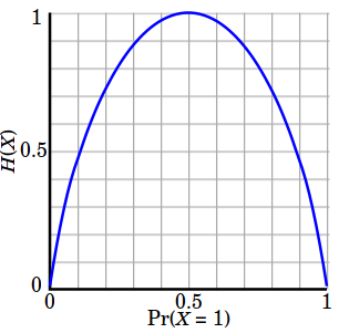
- Entropy of a group in which all examples belong to the same class: $$ entropy = -1 \log_2 1 = 0 $$ This is not a good set for training.
- entropy of a group with 50% in either class: $$ entropy = -0.5 \log_2 0.5 - 0.5 \log_2 0.5 = 1 $$ This is a good set for training.
So, basically, the entropy attempts to maximize the mutual information (by constructing a equal probability node) in the decision tree.
Similar to entropy, the Gini index is maximal if the classes are perfectly mixed, for example, in a binary class:
$$ Gini = 1 - (p_1^2 + p_2^2) = 1-(0.5^2+0.5^2) = 0.5$$Using a decision algorithm, we start at the tree root and split the data on the feature that results in the largest information gain (IG).
We repeat this splitting procedure at each child node down to the empty leaves. This means that the samples at each node all belong to the same class.
However, this can result in a very deep tree with many nodes, which can easily lead to overfitting. Thus, we typically want to prune the tree by setting a limit for the maximum depth of the tree.
Basically, using IG, we want to determine which attribute in a given set of training feature vectors is most useful. In other words, IG tells us how important a given attribute of the feature vectors is.
We will use it to decide the ordering of attributes in the nodes of a decision tree.
The Information Gain (IG) can be defined as follows:
$$ IG(D_p) = I(D_p) - \frac{N_{left}}{N_p}I(D_{left}) - \frac{N_{right}}{N_p}I(D_{right})$$where $I$ could be entropy, Gini index, or classification error, $D_p$, $D_{left}$, and $D_{right}$ are the dataset of the parent, left and right child node.
In this section, we'll get IG for a specific case as shown below:
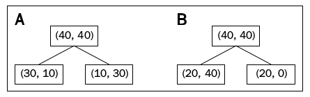
First, IG with Classification Error ($IG_E$):
$$ Classification Error = 1-\max p_j$$ $$ I_E(D_p) = 1 - \frac{40}{80} = 1 - 0.5 = 0.5 $$ $$ A:I_E(D_{left}) = 1 - \frac{30}{40} = 1 - \frac34 = 0.25 $$ $$ A:I_E(D_{right}) = 1 - \frac{30}{40} = 1 - \frac34 = 0.25 $$ $$ IG(D_p) = I(D_p) - \frac{N_{left}}{N_p}I(D_{left}) - \frac{N_{right}}{N_p}I(D_{right})$$ $$ A:IG_E = 0.5 - \frac{40}{80} \times 0.25 - \frac{40}{80} \times 0.25 = 0.5 - 0.125 - 0.125 = \color{blue}{0.25}$$ $$ B:I_E(D_{left}) = 1 - \frac{40}{60} = 1 - \frac23 = \frac13 $$ $$ B:I_E(D_{right}) = 1 - \frac{20}{20} = 1 - 1 = 0 $$ $$ B:IG_E = 0.5 - \frac{60}{80} \times \frac13 - \frac{20}{80} \times 0 = 0.5 - 0.25 - 0 = \color{blue}{0.25}$$The information gains using the classification error as a splitting criterion are the same (0.25) in both cases A and B.
IG with Gini index ($IG_G$):
$$ Gini = 1-\sum_jp_j^2$$ $$ I_G(D_p) = 1 - \left( \left(\frac{40}{80} \right)^2 + \left(\frac{40}{80}\right)^2 \right) = 1 - (0.5^2+0.5^2) = 0.5 $$ $$ A:I_G(D_{left}) = 1 - \left( \left(\frac{30}{40} \right)^2 + \left(\frac{10}{40}\right)^2 \right) = 1 - \left( \frac{9}{16} + \frac{1}{16} \right) = \frac38 = 0.375 $$ $$ A:I_G(D_{right}) = 1 - \left( \left(\frac{10}{40}\right)^2 + \left(\frac{30}{40}\right)^2 \right) = 1 - \left(\frac{1}{16}+\frac{9}{16}\right) = \frac38 = 0.375 $$ $$ A:I_G = 0.5 - \frac{40}{80} \times 0.375 - \frac{40}{80} \times 0.375 = \color{blue}{0.125} $$ $$ B:I_G(D_{left}) = 1 - \left( \left(\frac{20}{60} \right)^2 + \left(\frac{40}{60}\right)^2 \right) = 1 - \left( \frac{9}{16} + \frac{1}{16} \right) = 1 - \frac59 = 0.44 $$ $$ B:I_G(D_{right}) = 1 - \left( \left(\frac{20}{20}\right)^2 + \left(\frac{0}{20}\right)^2 \right) = 1 - (1+0) = 1 - 1 = 0 $$ $$ B:I_G = 0.5 - \frac{60}{80} \times 0.44 - 0 = 0.5 - 0.33 = \color{blue}{0.17} $$So, the Gini index favors the split B.
IG with Entropy ($IG_H$):
$$ Entropy = -\sum_jp_j\log_2p_j$$ $$ I_H(D_p) = - \left( 0.5\log_2(0.5) + 0.5\log_2(0.5) \right) = 1 $$ $$ A:I_H(D_{left}) = - \left( \frac{30}{40}\log_2 \left(\frac{30}{40} \right) + \frac{10}{40}\log_2 \left(\frac{10}{40} \right) \right) = 0.81 $$ $$ A:I_H(D_{right}) = - \left( \frac{10}{40}\log_2 \left(\frac{10}{40} \right) + \frac{30}{40}\log_2 \left(\frac{30}{40} \right) \right) = 0.81 $$ $$ A:IG_H = 1 - \frac{40}{80} \times 0.81 - \frac{40}{80} \times 0.81 = \color{blue}{0.19} $$ $$ B:I_H(D_{left}) = - \left( \frac{20}{60}\log_2 \left(\frac{20}{60} \right) + \frac{40}{60}\log_2 \left(\frac{40}{60} \right) \right) = 0.92 $$ $$ B:I_H(D_{right}) = - \left( \frac{20}{20}\log_2 \left(\frac{20}{20} \right) + 0 \right) = 0 $$ $$ B:IG_H = 1 - \frac{60}{80} \times 0.92 - \frac{20}{80} \times 0 = \color{blue}{0.31} $$So, the entropy criterion favors B.
In this section, we'll plot the three impurity criteria we discussed in the previous section:
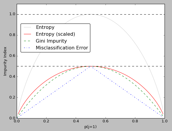
Note that we introduced a scaled version of the entropy (entropy/2) to emphasize that the Gini index is an intermediate measure between entropy and the classification error.
The code used for the plot is as follows:
import matplotlib.pyplot as plt
import numpy as np

def gini(p):
   return (p)*(1 - (p)) + (1 - p)*(1 - (1-p))

def entropy(p):
   return - p*np.log2(p) - (1 - p)*np.log2((1 - p))

def classification_error(p):
   return 1 - np.max([p, 1 - p])

x = np.arange(0.0, 1.0, 0.01)
ent = [entropy(p) if p != 0 else None for p in x]
scaled_ent = [e*0.5 if e else None for e in ent]
c_err = [classification_error(i) for i in x]

fig = plt.figure()
ax = plt.subplot(111)

for j, lab, ls, c, in zip(
      [ent, scaled_ent, gini(x), c_err],
      ['Entropy', 'Entropy (scaled)', 'Gini Impurity', 'Misclassification Error'],
      ['-', '-', '--', '-.'],
      ['lightgray', 'red', 'green', 'blue']):
   line = ax.plot(x, j, label=lab, linestyle=ls, lw=1, color=c)

ax.legend(loc='upper left', bbox_to_anchor=(0.01, 0.85),
         ncol=1, fancybox=True, shadow=False)

ax.axhline(y=0.5, linewidth=1, color='k', linestyle='--')
ax.axhline(y=1.0, linewidth=1, color='k', linestyle='--')

plt.ylim([0, 1.1])
plt.xlabel('p(j=1)')
plt.ylabel('Impurity Index')
plt.show()
Machine Learning with scikit-learn
scikit-learn installation
scikit-learn : Features and feature extraction - iris dataset
scikit-learn : Machine Learning Quick Preview
scikit-learn : Data Preprocessing I - Missing / Categorical data
scikit-learn : Data Preprocessing II - Partitioning a dataset / Feature scaling / Feature Selection / Regularization
scikit-learn : Data Preprocessing III - Dimensionality reduction vis Sequential feature selection / Assessing feature importance via random forests
Data Compression via Dimensionality Reduction I - Principal component analysis (PCA)
scikit-learn : Data Compression via Dimensionality Reduction II - Linear Discriminant Analysis (LDA)
scikit-learn : Data Compression via Dimensionality Reduction III - Nonlinear mappings via kernel principal component (KPCA) analysis
scikit-learn : Logistic Regression, Overfitting & regularization
scikit-learn : Supervised Learning & Unsupervised Learning - e.g. Unsupervised PCA dimensionality reduction with iris dataset
scikit-learn : Unsupervised_Learning - KMeans clustering with iris dataset
scikit-learn : Linearly Separable Data - Linear Model & (Gaussian) radial basis function kernel (RBF kernel)
scikit-learn : Decision Tree Learning I - Entropy, Gini, and Information Gain
scikit-learn : Decision Tree Learning II - Constructing the Decision Tree
scikit-learn : Random Decision Forests Classification
scikit-learn : Support Vector Machines (SVM)
scikit-learn : Support Vector Machines (SVM) II
Flask with Embedded Machine Learning I : Serializing with pickle and DB setup
Flask with Embedded Machine Learning II : Basic Flask App
Flask with Embedded Machine Learning III : Embedding Classifier
Flask with Embedded Machine Learning IV : Deploy
Flask with Embedded Machine Learning V : Updating the classifier
scikit-learn : Sample of a spam comment filter using SVM - classifying a good one or a bad one
Machine learning algorithms and concepts
Batch gradient descent algorithmSingle Layer Neural Network - Perceptron model on the Iris dataset using Heaviside step activation function
Batch gradient descent versus stochastic gradient descent
Single Layer Neural Network - Adaptive Linear Neuron using linear (identity) activation function with batch gradient descent method
Single Layer Neural Network : Adaptive Linear Neuron using linear (identity) activation function with stochastic gradient descent (SGD)
Logistic Regression
VC (Vapnik-Chervonenkis) Dimension and Shatter
Bias-variance tradeoff
Maximum Likelihood Estimation (MLE)
Neural Networks with backpropagation for XOR using one hidden layer
minHash
tf-idf weight
Natural Language Processing (NLP): Sentiment Analysis I (IMDb & bag-of-words)
Natural Language Processing (NLP): Sentiment Analysis II (tokenization, stemming, and stop words)
Natural Language Processing (NLP): Sentiment Analysis III (training & cross validation)
Natural Language Processing (NLP): Sentiment Analysis IV (out-of-core)
Locality-Sensitive Hashing (LSH) using Cosine Distance (Cosine Similarity)
Artificial Neural Networks (ANN)
[Note] Sources are available at Github - Jupyter notebook files1. Introduction
2. Forward Propagation
3. Gradient Descent
4. Backpropagation of Errors
5. Checking gradient
6. Training via BFGS
7. Overfitting & Regularization
8. Deep Learning I : Image Recognition (Image uploading)
9. Deep Learning II : Image Recognition (Image classification)
10 - Deep Learning III : Deep Learning III : Theano, TensorFlow, and Keras
Ph.D. / Golden Gate Ave, San Francisco / Seoul National Univ / Carnegie Mellon / UC Berkeley / DevOps / Deep Learning / Visualization